In the event that any external links are broken or outdated please let me know as soon as possible.

From Newton to Kinematics:

The question of what you learn and how you, as the student, integrate this into your thinking keeps a large group of physics teachers very occupied across the country. Do we do this first or that? Are calculators helpful or do they prevent the development of conceptual understanding? Is that topic really important or is it just traditional? For me the question of whether to start with dynamics or kinematics is one of these questions. The tradition is that we start with kinematics because it allows us to explore your understanding of plots and the material you learned in Calculus I (Differentiation) while also stressing your algebra skills. All seems well and good except that in the end that's not normally how we figure out to describe the behavior of an object. More typically we apply Newton's Laws to understand what causes it to move and then compare those expectations to what we actually see. We have started by considering Newton's Laws (mostly in just 1 direction) and now the question is how can we extract the predicted behavior of the object from that analysis? This also has strong connections to what you are learning, or possibly have learned, in Calculus II (Integration). Here we go....from most basic to more complicated....

Starting with 'a' from Newton's 2nd Law:

As we go through this review of plots and their meaning in the world we will start with what it might mean if it describes acceleration first. This is because the acceleration is what we learn from our Newtonian analysis of the forces. From there we can work towards velocity and position. It is also important to recognise that if we know the acceleration we have some information about Fnet which tells us something about the forces on our freebody diagram. This is why we need to have a clear understanding of the slope of a function (derivative) and the area under the function (integral) for physics. For simple linear and quadratic functions we can probably survive without the machinery of calculus but we use it as a way to practice these potentially 'new' skills.

General Approach: Review

The first section of this breadcrumb is hoped to be a review of your skills at interpreting graphs/plots of acceleration, velocity, and position. This interpretation connects with MTH 251 calculus but can also be understood from a more algebraic perspective. We may not explore all of the activities while in class due to limitations of time but it is expected that all of the graphical stuff makes sense to everyone.

With each plot we will first ask what it might mean if the plot describes acceleration, velocity, or position as a function of time.

Then we will explore what the slope tells us about the behavior through time. The primary tool to develop that understanding are the units of the slope.

Then we will ask if the integral of the function (area under the plot) indicates about the behavior through time. Again, the primary tool to develop understanding will be the units of the area.

Generic Plot I:

Below is a generic plot that relates two variables. For the time being we will choose 'Variable 1' to be time and 'Variable II' to be acceleration, velocity, or position in 1D (call it the x direction for starters).

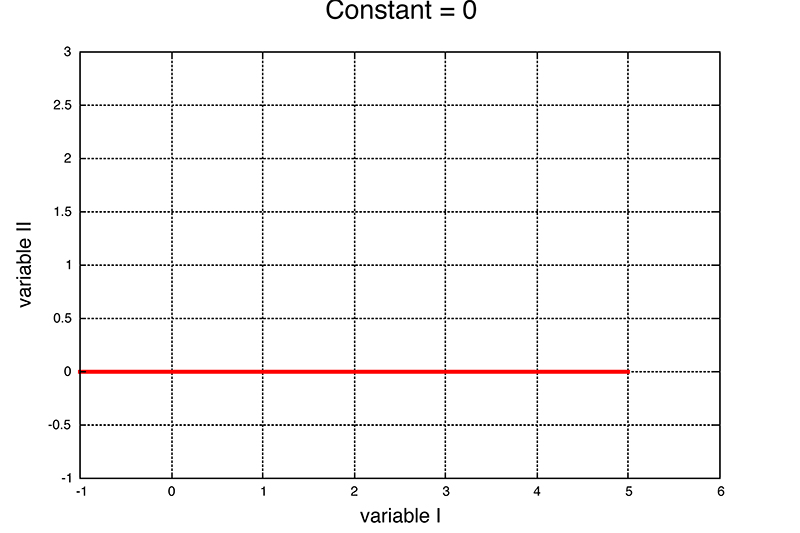
Activity: This plot is describing the motion of an object in one direction. See if you can verbally describe various features of the motion represented by the plot.

What does shape of the plot (flat line) 'say' about how the object is moving when 'Variable II' is acceleration, velocity, position? In each case be clear about whether the object is speeding up, slowing down, moving, not moving, and where it starts and finishes in the x direction?

We will gather as a class to discuss briefly and then return to our groups to consider another feature of this plot - the slope. We'll talk about the units of the slope in a moment when there is a non-zero slope.

What does slope of the plot (flat line) 'say' about how the object is moving when 'Variable II' is acceleration, velocity, position? In each case be clear about whether the object is speeding up, slowing down, moving, not moving, and where it starts and finishes in the x direction? Is the slope meaningless in any of these cases?

There is no area under this curve so it's a little unclear what the integral might mean -- that will come up in a moment.

Generic Plot II:

We will continue to choose 'Variable 1' to be time and 'Variable II' to be acceleration, velocity, or position in 1D.

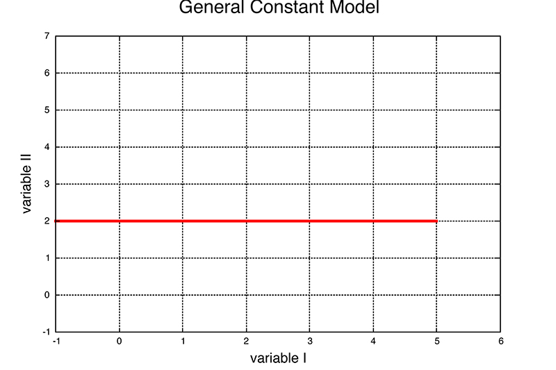
Activity: This plot is describing the motion of an object in one direction. See if you can verbally describe various features of the motion represented by the plot in this case.

What does shape of the plot (flat line) 'say' about how the object is moving when 'Variable II' is acceleration, velocity, position? In each case be clear about whether the object is speeding up, slowing down, moving, not moving, and where it starts and finishes in the x direction?

We will gather as a class to discuss briefly and then return to our groups to consider another feature of this plot - the slope. We'll talk about the units of the slope in a moment when there is a non-zero slope.

What does slope of the plot (flat line) 'say' about how the object is moving when 'Variable II' is acceleration, velocity, position? In each case be clear about whether the object is speeding up, slowing down, moving, not moving, and where it starts and finishes in the x direction? Is the slope meaningless in any of these cases?

We will gather as a class to discuss briefly and then return to our groups to consider another feature of this plot - the area under the curve.

Area Under Curve: Units

Because the line describing the motion is above the horizontal axis there is an area between the horizontal axis and the plot. Since area is H (height) x W (width), each of which has units, we can determine the units of the area.This tells us the meaning of the area under the plot, between two times.

If the vertical axis is acceleration then H has units of m/s2 and W has units of s (time). That means the area 'under the plot' has units of m/s which is a velocity.

For a velocity plot the H has units of m/s and the W has units of s. The area has units of m which is a position or change in position.

Finally, on a position plot, the area has units of m s. There isn't any meaningful property of the motion of an object which has units of m s. This tells us that the area under a position plot has no physical meaning at this time.

We will gather as a class to discuss briefly and then return to our groups to consider another feature of this plot - the slope. We'll talk about the units of the slope in a moment when there is a non-zero slope.

What does area 'under' the plot (flat line) between two times 'say' about how the object is moving when 'Variable II' is acceleration, velocity, position? In each case be clear about whether the object is speeding up, slowing down, moving, not moving, and where it starts and finishes in the x direction?

We will gather as a class to discuss briefly your perspectives.

Generic Plot III:

We will continue to choose 'Variable 1' to be time and 'Variable II' to be acceleration, velocity, or position in 1D.

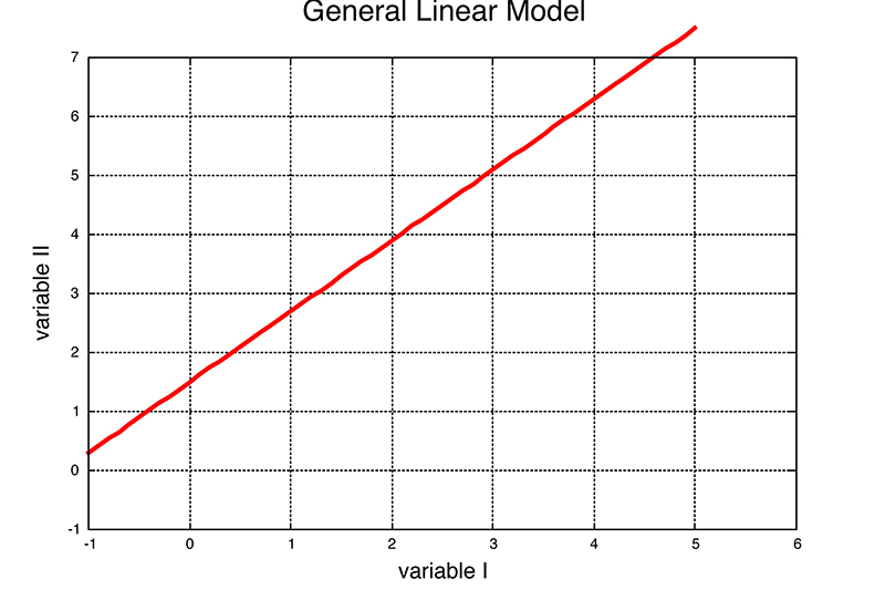
Activity: This plot is describing the motion of an object in one direction. See if you can verbally describe various features of the motion represented by the plot in this case.

What does shape of the plot (flat line) 'say' about how the object is moving when 'Variable II' is acceleration, velocity, position? In each case be clear about whether the object is speeding up, slowing down, moving, not moving, and where it starts and finishes in the x direction?

We will gather as a class to discuss briefly and then return to our groups to consider another feature of this plot - the slope.

Slope of a Curve: Units

Slope is defined to be 'rise over run' or slope = rise/run. So lets look at the units of the slope in each case.

If the vertical axis is acceleration then the 'rise' has units of m/s² and the 'run' has units of s (time). That means the slope of the acceleration plot has units of m/s³ which not a physical quantity most of us have a name for at this point. Some of you may know that it is sometimes called the 'jerk' (as in whiplash).

For a velocity plot the 'rise' has units of m/s and the 'run' has units of s. The slope has units of m/s² which is an acceleration. Most (many) of you know this but my point here is that this is how we identify the meaning of features on a plot when it's a new and unknown type of plot.

Finally, on a position plot, the 'rise' has units of m and the run has units of s. The slope has units of m/s which is a velocity as most of you know.

What does slope of the plot (flat line) 'say' about how the object is moving when 'Variable II' is acceleration, velocity, position? In each case be clear about whether the object is speeding up, slowing down, moving, not moving, and where it starts and finishes in the x direction? Is the slope meaningless in any of these cases?

We will gather as a class to discuss briefly and then return to our groups to consider the other feature of this plot - the area under the curve.

What does area 'under' the plot (flat line) between two times 'say' about how the object is moving when 'Variable II' is acceleration, velocity, position? In each case be clear about whether the object is speeding up, slowing down, moving, not moving, and where it starts and finishes in the x direction?

We will gather as a class to discuss briefly and then talk a bit about geometric methods for determining the precise area under a linear plot like this. It includes both rectangles and triangles but is fairly direct.

Practice Graph:

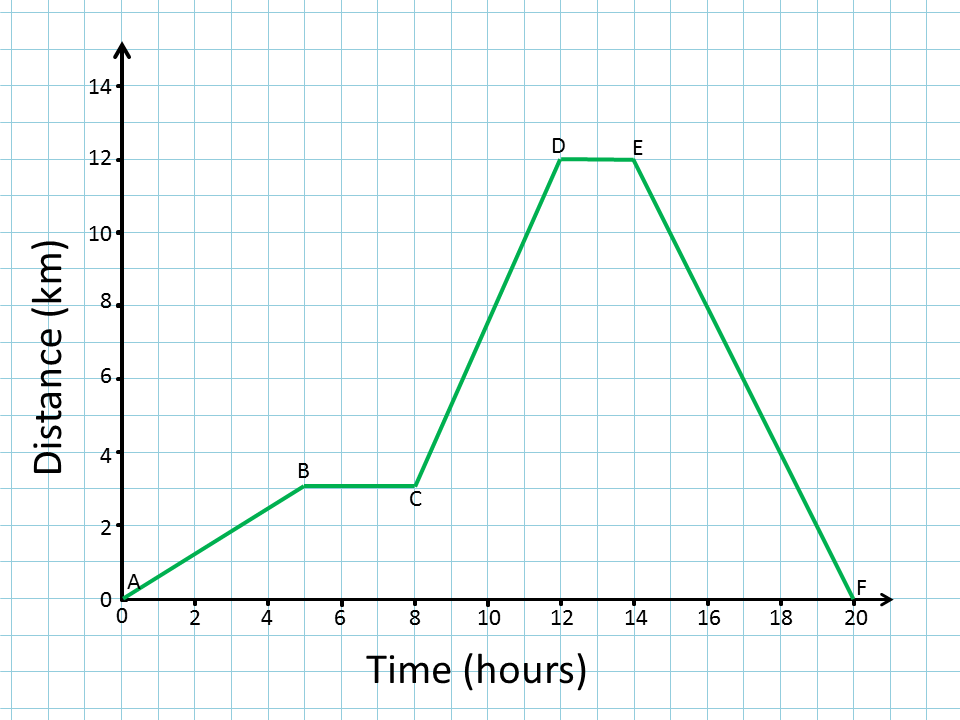
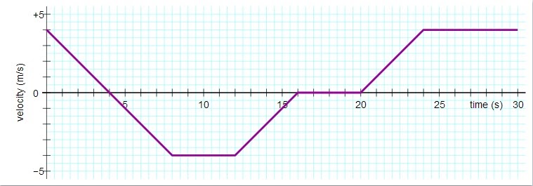
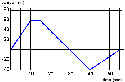
Consider how you would interpret the following graph both as a position - time graph AND as a velocity - time graph by changing the units. If you are comfortable with this then you are ready for the HW. In every interval you should be able to describe the velocity, the acceleration, and the change in position.

HW: Kinematics I

There are 5 intervals on this graph representing different behaviors of an object. For each interval determine the velocity and acceleration of the object as well as the distance traveled. Be careful about units.

HW: Kinematics I

Using the same graph above re-label the axes as follows. The vertical axis is velocity in m/s and the horizontal axis is time in s. For each interval determine the acceleration of the object as well as the distance traveled. Be careful about units.

HW: Kinematics I

For this graph determine the final position of the object assuming it starts at a location called 0. You need to 'integrate' this graph by finding the area in each section geometrically.

t

Thanks to Paul Blomenberg at Luthern HS in CO for the use of the image. 

From an Integration Perspective: MTH 252

For this class I don't need you to be able to reproduce the integration processes illustrated below. I want you to see them because, ultimately, this is how we actually solve physics and engineering problems. We start with the acceleration function and integrate it. Many of you are in MTH 252 and you will see some or all this integration process soon. I want to have an awareness of how it is connected to the physics. Some of you already have some basic integration skills and I want you to see how integration works in an applied setting.

Ultimately I need you to know the results of these integration settings and, more importantly, the conditions under which they apply. Everything that we do in this process hopefully makes sense from comparing the results of the integration to the discussions about the meanings of the 3 plots we have just reviewed.

Acceleration Plot: Generic Plot I

Assuming this is an acceleration plot......

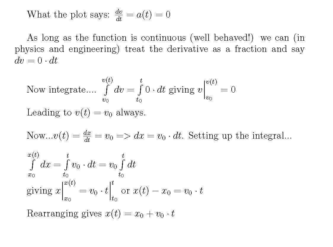
This is just the same thing you've learned a dozen times in different forms. Distance = rate * time! The form above is the more standard version for physics and arises naturally from integrating the acceleration from Newton's 2nd Law in the special case where a = 0.

Take Home:

when a = 0, then x(t) = x₀ + v₀ ^. (t- t₀) and v(t) = v₀

NOTE:

You may have noticed that all of the integrals above are definite integrals. The general approach in math class is to think mostly in terms of indefinite integrals but in science and engineering we more commonly are applying the math to a setting with defined limits. As a result definite integrals are more common. This eliminates the concern about the integration constant that you will learn about.

Acceleration Plot: Generic Plot II

Starting with the interpretation that this is an acceleration plot....

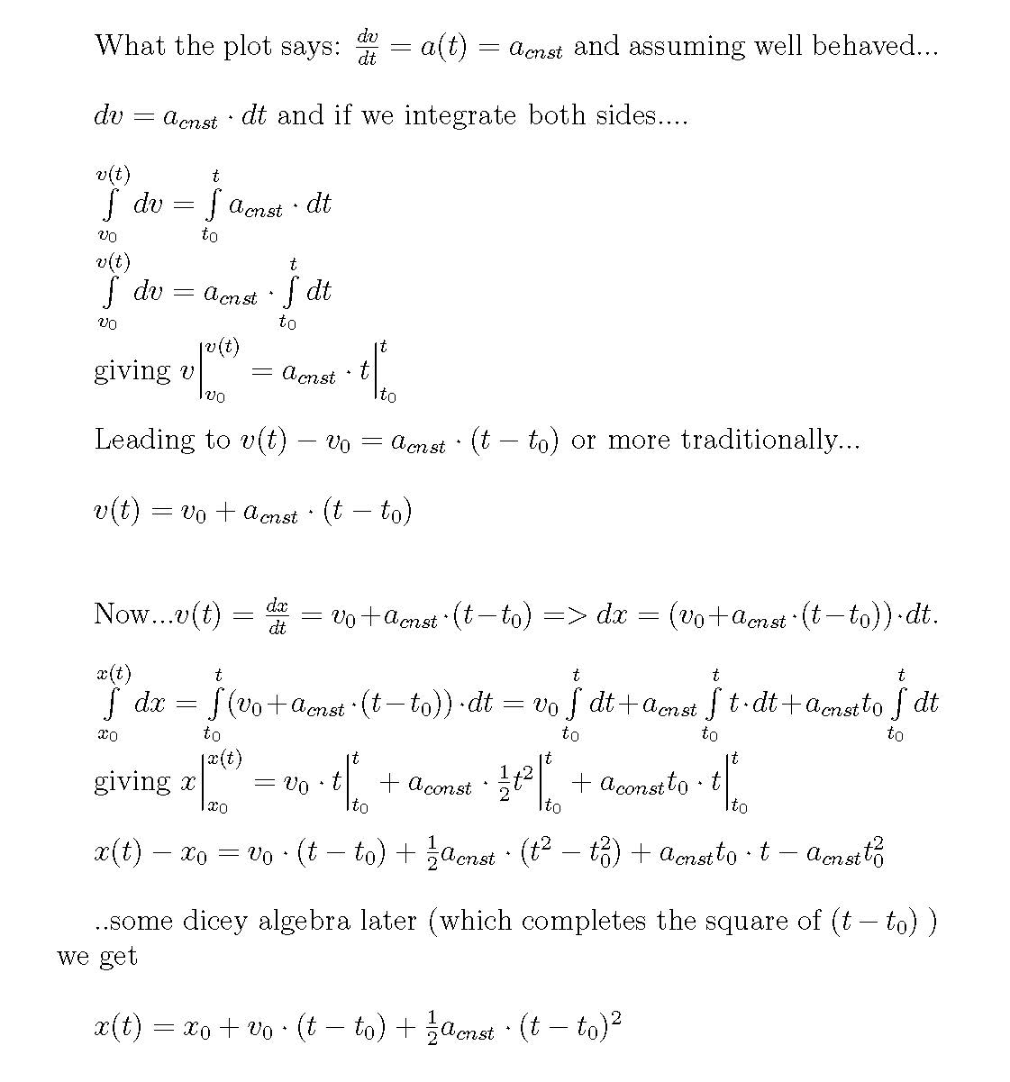
This is a bit more complex that distance = rate x time. The person in the street does not carry around a mathematical model for the distance covered while constantly accelerating but now you have such a tool.

Take Home:

when a_c = constant then,

v(t) = v₀ + a_c ^. (t- t₀)

x(t) = x₀ + v₀ ^. (t- t₀) + 0.5 a_c ^. (t- t₀)²

 

Acceleration Plot: Generic Plot III

Starting with the interpretation that this is an acceleration plot....

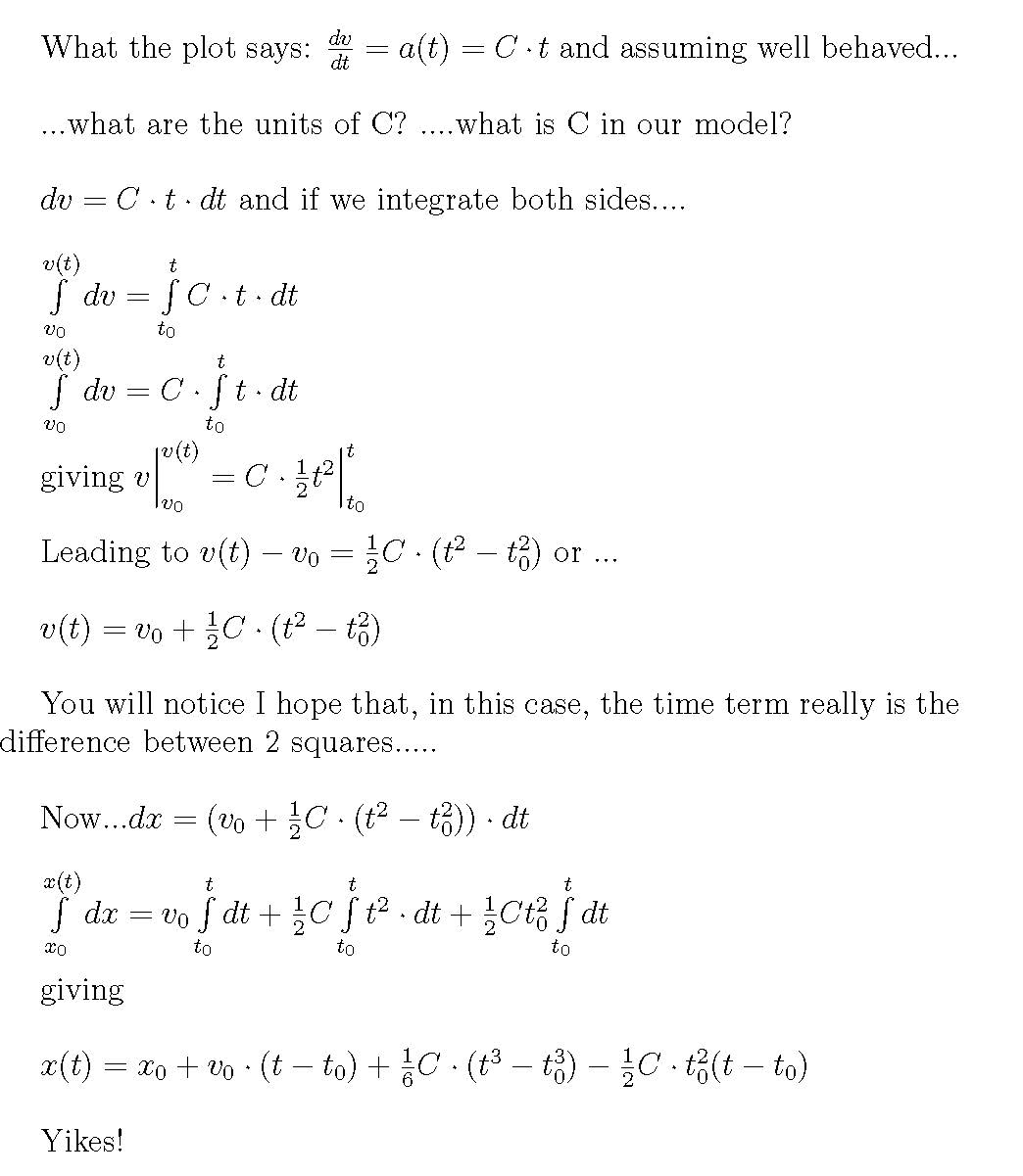
Yikes is right! When the acceleration is NOT constant it is better not to worry about analytic solutions and approach each problem as a unique integration problem in a particular setting. This is the domain of ENGR 212 Dynamics for students on the physics or engineering track.

Take Home:

when a = a(t) save it for next year!

These are the tools that will let us describe how any object will move once we know what it's acceleration is. It can get complicated but the process always works......with practice.

Assignment: HW: Kinematics I

Turn in the various (2 with many parts) homework problems in this breadcrumb. For these problems please use the problem solving format described in the Concepts breadcrumb. The plot which you are analyzing should be clearly present in your solution and will probably be noticeably annotated.

Assignment: Reading

Next we move on to crafting a structured approach to using mathematical tools to describe the kinematics of an object when a = 0 or a = constant. Move on to the Kinematics Practice Breadcrumb.